End-to-end Keyword Bidding for Apple Search Ads

Canva’s performance marketing team has many digital marketing channels that we use to help new users discover Canva, and highlight new features to returning users. One of the channels, Apple Search Ads (ASA), is a marketing channel to target iOS users searching for apps in the Apple App Store. Advertisers set a maximum bid for each keyword in ASA and then adjust these bids based on the quality (how often users move through the funnel) and volume of the impressions they receive through the campaign.

Canva runs campaigns for ASA in many regions targeting keywords based on products (Magic Write), user intent (Background remover), and brands (Canva). This can add up to tens of thousands of keywords per campaign that need their bid price to be maintained. Moreover, Canva runs many of these campaigns over various regions around the world. This can be a complex and labor-intensive task, so the Marketing Optimization team looked to improve this workflow by automating it.

Apple, unlike Google and Meta, doesn’t provide an automated bidding product for managing these bids. After looking at other various third party solutions, our consensus was that it was better to build a system in-house so we could align it more efficiently with our marketing strategy.

Background and overview

Before launching into a description of our system, it’s helpful to understand some concepts about Apple Search Ads and some context about our previous system.

Why do we bid?

We are motivated by the desire to surface ads related to Canva using specific keyword choices on Apple Search Ads. We want these ads to attract new active users (we can use other metrics, such as high return on investment users, for instance). The system has to optimize on this metric primarily while controlling cost when it bids on keywords.

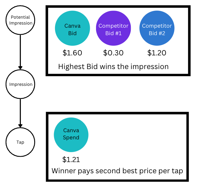
Apple Search Ads uses a (slightly modified) Vickrey auction system (also known as second price auction), which has the following characteristics:

• Impressions are won by the highest bidder.
• The bidder is only charged if the impression turns into a tap (quite literally, when a user taps on the ad).
• The bidder is charged the second highest bid price plus 1 cent, typically denominated in USD, but can be priced in local currency.

This is a popular auction system because it encourages bidders to bid the true value of the impression (called allocative efficiency) as they only win impressions at a price lower than their bid. Because a bidder is charged only on a per-tap basis, the second important metric for us is cost per tap.

Apple Search Ads allows advertisers to modify bids regularly. In practice, bids are usually updated only once a day, so bids affect the win and loss of many repeated auctions.

Our system would have to maximize the primary metric (e.g., return on ad spend), while minimizing the second metric (e.g., cost per tap), subject to a per week budget, to get the best bang for our buck.

Previous system

Canva’s initial system for managing these keywords was an SQL-based rules-based system using historical data to determine the keyword quality. Keywords are selected by marketers or by a keyword exploration system (which is a large project and out of scope here). We chose SQL because it could be implemented directly into the data warehouse. A reverse ETL job would update keyword bids in Apple Search Ads daily once the new bids have been calculated. We didn’t need to operate in real-time because our primary metric was insensitive to bid changes in a duration of less than a day.

This system relied on a simple multiplicative bid logic, where we calculate the bid multiplier as a function of keyword quality, which we multiply against the previous bid on a per-keyword basis. If the multiplier is a value greater than 1, we increase the bid. If the value was less than 1, we decrease the bid. We did this because it provided a quick way to automate and scale down the cost per tap because many keywords didn’t provide a return on ad spend. The bids were then updated the following day depending on the result of the previous day.

The system was significantly better than manually inputting a fixed value for each keyword, which the marketing team did. We rarely changed our bids, contributing to lower return on ad spend because every keyword (including many under-performing ones) were being bid on and won.

High-quality impressions led to the attributed keywords having bids increased, while keywords that didn’t meet quality thresholds had bids decreased. Over time, we would expect the best keywords to still win impressions and the others to lose, resulting in an efficient campaign spend.

The initial implementation of this system was successful. It was simple and quick to integrate with Apple Search Ads and led to immediate cost savings. Marketers felt the system was understandable and intuitive. It was also similar to how they would manage bids.

Unfortunately, this system has an Achilles heel: the information gained from low bids was less than would be gained from high bids. Apple Search Ads only reports back information about the number of won auctions, so when we get outbid, we don’t know by how much or how many impressions we could have won with a higher bid. The information disparity between winning and losing auctions means it's easier for the system to reduce bids than increase them.

After the initial success of the SQL-based feedback loop system, we found that the marketers would make manual changes to increase the bids on keywords they knew, based on domain knowledge, were high value. The many overrides caused instability in the system. Their frustration after the honeymoon period led to a rethink of our solution.

Why does the original SQL-based system break down? Here are the reasons:

• The requirements to bid down are easier than the requirements to bid up.
• This results in a system where only a few keywords are bid on and all others have very low bids.
• Unresponsive to competitor behavior: if a competitor starts bidding higher on a very high-quality keyword, and we win 0 impressions. We don’t have enough information to know how to increase our bids.

An ideal system would both:

• Explore: Bid at higher amounts irregularly to determine if there’s opportunity in outbidding competitors.
• Exploit: Bid at amounts most likely to result in the best return for the campaign as a whole.

This tradeoff between exploration and exploitation is difficult to build into an SQL-based system. Indeed, it was very good at exploitation but largely failed to explore opportunities.

Our New System Overview

Our requirements are as follows:

• We need to estimate, for each keyword, the return (this can be return on ad spend, internal company metrics, or a blend of these metrics via linear scalarization).
• The system has to converge around the reference budget, given by the weekly budget allocation for each campaign.
• Allow for the system to explore and exploit opportunities if they present themselves.
• Provide a level of explainability to stakeholders, who can see what’s happening in the background from time to time.

Our new system is a contextual multi-armed bandit (CMAB) system. We can use CMABs to engage with this Exploration-Exploitation problem. We chose to use that for this problem, inspired by an excellent writeup by the marketing automation team at Lyft. While there are similarities between their system and ours, fundamentally, we’re solving a very different problem. The Lyft system is more general and optimizes a two-side marketplace to acquire riders and drivers. Our system is an end-to-end system for a specific channel, although it can be extended to other channels in the future.

The CMAB looks to find the best combination of ways to move the levers of keyword bids in a campaign to maximize the return and maintain a spend near the budget amount.

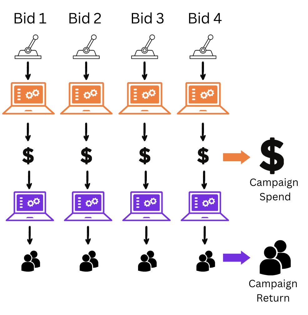
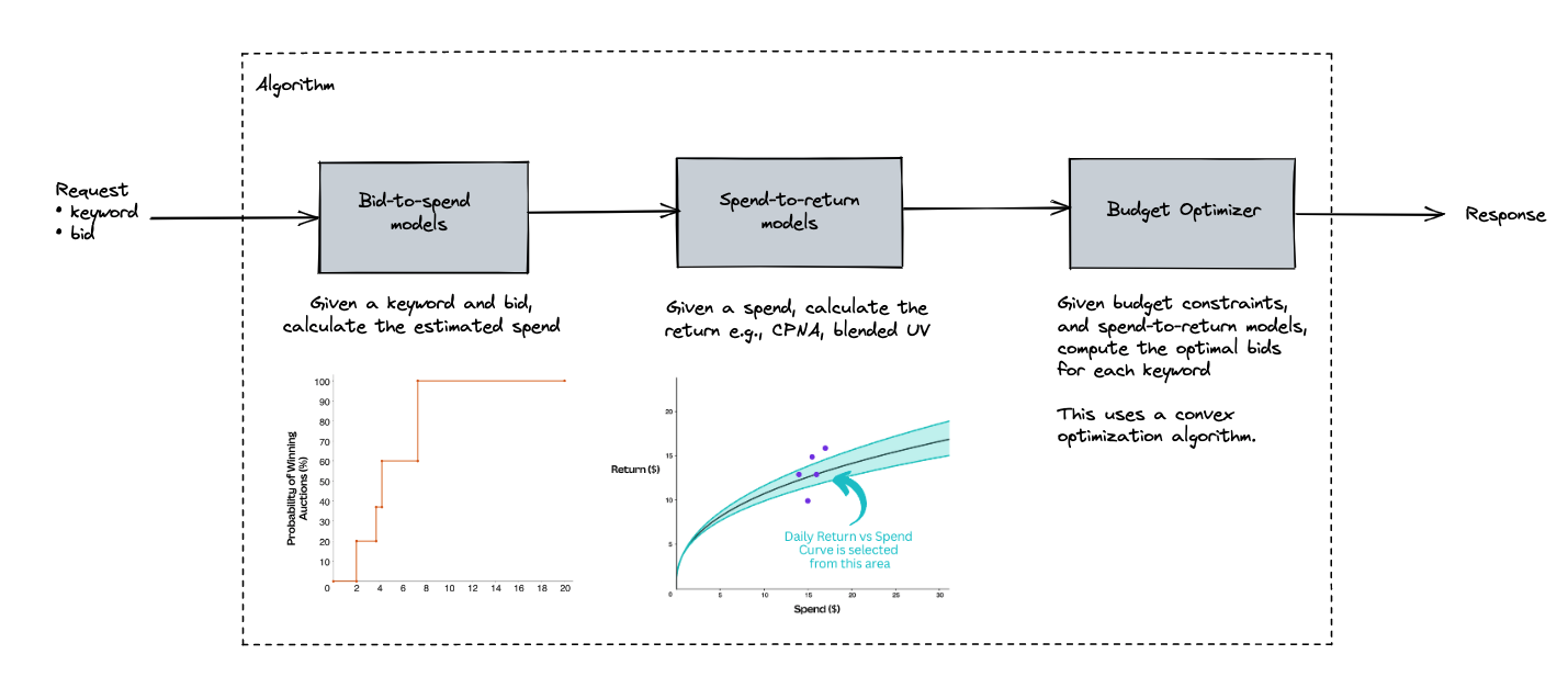
This means we need three parts to build an improved system:

• Accurately predict the bid amount (per keyword in each campaign) that will get us close to a certain spend.
• Accurately predict the return each keyword will make at different spend amounts.
• An optimization algorithm that can find the best spends to achieve the objective, given that each campaign has a daily average budget spend target.

You may see this as a closed-loop control system where we need to meet the average budget spend target per week while maximizing returns, and you would be right! There are many different ways of approaching the above problem, each with its own strengths and weaknesses. Our design is well-suited in the context of Canva, which we sketch below.

Bid Amount and Spend Model

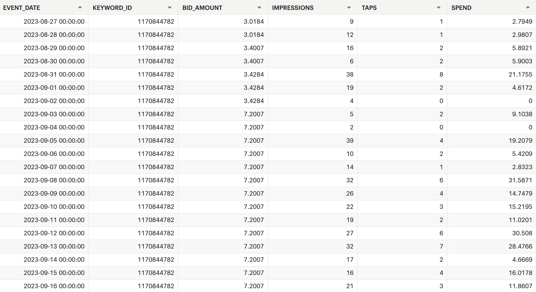
We know that the number of impressions we win on a given day is based on Canva’s bid and other bidders. We also know we will only spend on a keyword if a user taps on the ad. When there’s a spend, we get a direct observation of the return of the keyword. Remember that some keywords have low performance, so we want to make sure we don’t bid on these keywords over time if we know for certain that they don’t contribute to reward.

This means we can infer the range of the competitor’s bid based on the number of impressions we win each day:

• If we receive significantly fewer impressions than usual, it implies the highest competitor bids are greater than ours.
• If we receive significantly more impressions than usual, it implies we have the highest bids as a proportion of our number of bids. We can also estimate our spend based on the number of taps we observed for a keyword from historical records.

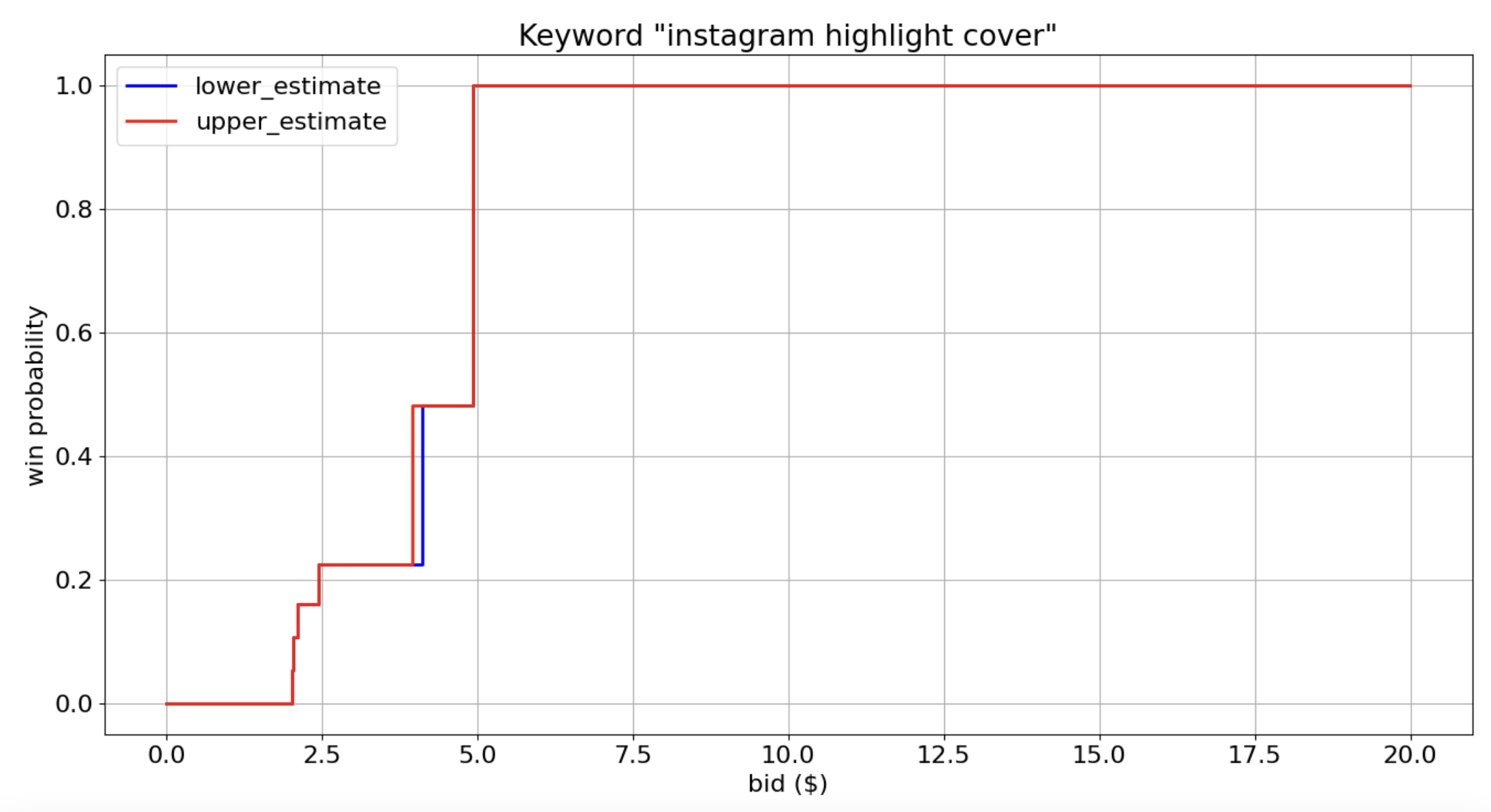
When we know the range of values but not the true number, we can use survival analysis to estimate the probability that the bid will be the highest.

We need only focus on the second-highest competitor’s bid (price) on any keyword we’re interested in for any auction round. When our bid is lower than the second-highest competitor, we know we didn’t win. Our bid needs to be higher than the winner’s bid by 1 cent to win. This is when we have right censoring.

When we win a bid, however, it’s possible to have no taps despite having impressions. In this case we don’t have a direct observation of spend because we’re only charged on a per-tap basis. This is when we have left censoring.

We have interval-censored data because our bidding scenario has both left and right-censoring. In either case, we don’t know if we won or lost the bid, and therefore don’t have any record.

With this relationship between bid amount and win probability, we can estimate our actual spend at different bid amounts. To keep the model responsive to changes in our competitor’s bidding behavior, we use recency weighting, where we pay higher attention to the most recent data-points than older ones.

As our scenario has both left and right-censoring, we can’t use the classic Kaplan-Meier nonparametric estimator, which only deals with right censoring. Instead, we turn to a non-parametric expectation-maximization (EM) algorithm developed by Turnbull. We then fit this on each keyword to get a bid estimation model. We use the bid distribution from each keyword to estimate the expected taps (and equivalently, spend).

Another challenge is that we don’t get explicit feedback per bid attempt, but instead, we get the aggregated number of taps and spend for any keyword because ASA doesn’t provide this information. This makes it much more difficult to apply Turnbull’s algorithm unless only a single tap is observed. Turnbull’s algorithm needs a non-trivial bound as an estimate of the left censoring case, but the aggregation of the spend poses a challenge here. We get around this by using a tuned threshold on the average spend per tap for each keyword as the estimated left censored bound. We assume our competitors don’t have a wide spread in their bids, which works well in practice.

Since we can now estimate the amount of spend based on a bid per keyword, all that’s left is to estimate the return on a given level of spend for each keyword.

Spend-to-Return Model

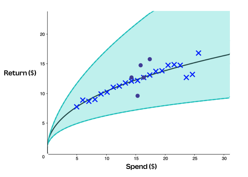
As discussed previously, the spend-to-return model needs to accurately predict the return on investment at different spend levels on different keywords. It needs to be flexible enough to handle significant changes in business requirements, so must be able to extrapolate to much higher or lower spends that are seen in the dataset. Additionally, because of the way we plan to solve for the most efficient spend values, we also want the function to be differentiable.

To model the relationship for each keyword under these requirements, we assume that the spend-to-return model should be parametric. However, the choice of parametric function needs to be informed based on our domain knowledge of the usual relationship between spend and return metrics. The spend-to-return model should obey the following:

• Non-decreasing: Increasing the spend doesn’t decrease the return.
• Diminishing returns: The gradient of the curve flattens out as spending increases.

We use a Hill function as our function curve for each keyword because it fits these criteria and also allows some additional hyperparameters to independently improve the fit for each campaign. We enforce (with two parameters, alpha and gamma) the diminishing returns on each of the keywords historical spend and returns to get a good approximation.

Explore-Exploit

One issue that can occur when using an automated system based on diminishing return curves is that the system can fixate on specific keywords. It will then bid the same amount on those keywords every day. As mentioned previously, this can cause some keywords never to win any bids, and we never get to see their potential performance. We could also paint ourselves into a corner by settling on a suboptimal bidding strategy.

Given that we want to spread our eggs into as many baskets and bid on as many keywords as possible instead of relying on a few good keywords, we need an automated way of increasing the diversity of our bids while not moving too far away from our perceived "optimal" behavior.

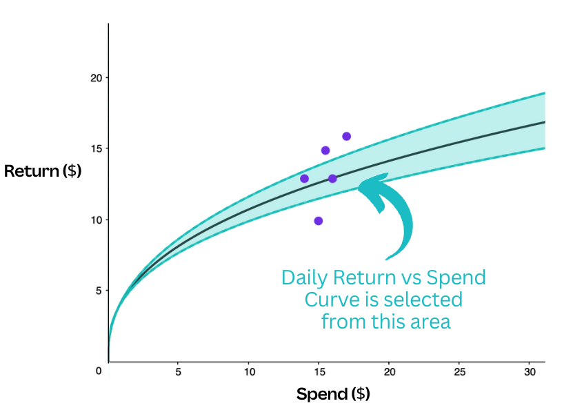
We introduce some variety with a technique called Thompson sampling. Instead of fitting a single curve to the data points, we fit a distribution of curves and sample a curve from this distribution each day. The spend-to-return curves for each keyword will vary slightly and look to have different optimal spend amounts each day. The distributions, however, have less variance for more reliable keywords (and have more data points), so the spend targets are similar. Conversely, keywords in which the system has less confidence have more variety and explore different spend values.

A Cold start problem

The main challenge with fitting spend-to-return distributions for each keyword is that some keywords have very low variety in spend levels or a low number of datapoints. It’s challenging to fit curves with a good ability to extrapolate to higher or lower spends.

The solution in this case, inspired by Lyft, is using a separate non-parametric model (LightGBM) that’s trained on every keyword in the dataset and then used as a prior for each keyword curve. We use this model’s predictions at a range of typical spend levels as "synthetic" data points that we can add to the actual data points for a keyword. We found that about 15-20 added to all keywords was sufficient to find a balance of accuracy for both old and new keywords.

We also fit a model for campaigns or regions to act as fallbacks if a keyword is added between training and inference time.

The result is that the Spend-to-Return is flexible enough to handle changes in business requirements and allow efficient extrapolation to much larger or smaller spends. It accounts for new keywords, keywords with little spend variety, and adds diversity to the spending behavior by design.

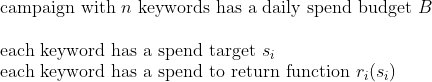
Keyword Spend Solver

When we have curves for all the keywords, we need a way to determine how much to spend based on the daily campaign budget. We can treat optimization in this case as a simple numerical optimization problem where the target is to maximize the return from a campaign constrained by not overspending the daily budget. Our optimization framing is as follows:

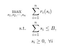
Since the campaign spend curves are designated to be differentiable, strictly increasing and have diminishing returns, the problem has exactly one unique global solution. We can solve it with an off-the-shelf numerical solver (in our case, we use L-BFGS) even when the number of keywords in a campaign is in the tens of thousands.

We used a few tricks to improve the speed of the solver including:

• Moving from a hard constraint on the deviation from the campaign budget to one that allowed small deviations if it made the solution quicker (soft constraints). We don’t have to be exact in our solutions because the quick feedback on a per-day basis helps to bring the system to convergence.
• Pre-calculating first order derivatives so the solver doesn’t need to estimate this.
• Setting reasonable initial values for spends and setting some bounds on the maximum and minimum spends.

This resulted in a large speed-up over a constrained numerical solver.

Results

We’ve rolled out our system to a majority of our Apple Search Ad campaigns since November 2022. It maintains models for nearly 10,000 keywords across 11 campaigns. Since rolling out the system, the campaigns are able to achieve spend and quality targets much more regularly with less full-time employee effort.

Our system demonstrated strong performance with a reduced cost compared to the primary metric of new active users we were aiming for, with between 5% and 50% cost reductions depending on the campaign. In contrast to the previous system, our new system was capable of exploring and exploiting keywords, thus overcoming the weaknesses of the previous system.

It’s extremely responsive to changes in campaign budgets, and can make changes to keyword bids if the campaign budgets go through radical changes (sometimes reducing or increasing by 50%) in a matter of days. This has allowed us to scale up or down new campaigns very quickly while maintaining a high level of efficiency. There would be a significant time cost if we had to do this manually.

We’ve also developed a user-friendly interface for marketers to feed campaign budget data and monitor system performance. This is important when explaining to stakeholders what the system is doing, and when we’re debugging issues with the system.

Initially, it took us about 6 hours to train and score all keywords. With subsequent improvements, and workflow optimizations, we reduced this by 50%. The biggest improvement was because of parallel training of each bid-to-spend model from a previously sequential training scheme.

From a maintainability perspective, because the system is divided into three parts, it’s much easier to maintain and improve on each component separately. For instance, we can work on improving the spend-to-return forecasting without having to make changes to the bid-to-spend model. However, note that while each component is independent in the codebase, the whole system is not. As such, testing does require end-to-end integration testing.

Future

This system doesn’t account for other factors that can impact spend and quality metrics, for example Canva events like Canva Create, day of the week traffic, and so on. These might be once off, or periodically occurring events. We can exploit them by bidding on keywords associated with these events. We plan to improve our forecasting ability by taking these into account.

At present, we set a steady daily budget each day, but in theory we would want to pace that budget out based on previous days results and known periods of higher traffic. Ideally, we would have a budget pacing system to reduce target spends if we’re over budget and vice versa.

Since deploying this system, new metrics are available through Apple Search Ads dashboard that would be useful to integrate into the model, including impression share estimates. The additional information would help the spend model improve its estimation of return.

Finally, we plan to explore a multi-objective version because typically each campaign has a different objective. We want to be able to find a Pareto front on these campaigns to optimize the overall set of campaigns based on a few primary metrics.

Acknowledgements

We would like to thank James Law, our Group Product Manager who led a lot of the discussions and provided an immense amount of support, and Dior Kappatos and Yann Fassbender, our supportive stakeholders. We would also like to give a shoutout to our ML Platform for providing us with a reliable platform and tools to improve our bidding system.

Interested in building scalable machine learning systems? Join Us!