Machine Learning
Deep Learning for Infinite (Multi-Lingual) Keywords
How we used a CLIP-inspired model to suggest keywords for template labeling in multiple languages.

At Canva we have millions of pieces of content, across many languages to serve our over 100 million monthly active users around the world(opens in a new tab or window).
In order for them to be surfaced during search, keywords are a necessity. It is common practice in most websites to include keywords in order to be indexed on search engines. Our in-house search engine powering the editor (as seen below) relies on good keywords to bring up the most relevant content. The lack of keywords on a piece of content can also affect its surfacing on the editor during a user's design session.

Canva has a marketplace for creators(opens in a new tab or window) which allows creators from around the globe to earn a passive income by earning royalties from templates and design elements such as photos, illustrations and many more listed on the marketplace.
While the most experienced designers know which keywords are suitable, it is a guessing game for some of our newer creators. This means that the learning curve for newer creators is steep, as they would need to master this as well as create aesthetic templates and content. Moreover, these keywords need to be in multiple languages to cater to Canva's diverse user base.
In order to let the creators focus on creating, and less on keywords we developed a deep learning model to speed up the process of keyword selection.
In this blog, we will go through how we gathered the data, designed the model architecture, trained with the special loss function that we chose, and finally discuss the results.
Model Architecture and Training
Typical classification models are only capable of classifying a
predetermined number of classes. The usual approach is to one hot encode
the labels. By denoting labels with numbers, we destroy any relationship
between the labels, which are obvious when considering the names of
labels (e.g., shark, sharks). We could theoretically support an
infinite number of keywords, including in languages that it wasn't
specifically trained for.
Siamese Language Models
The model displayed below is by CLIP(opens in a new tab or window). It is denoted "siamese" since we use twin models which start off with same weights but will take in different inputs. The two components of the architecture are the
- Keyword embedding model: this is a multi-lingual sentence transformer that converts a suggested keyword into an embedding, and
- Title and text content embedding model: this is also a multi-lingual sentence transformer that converts the title and text content in a template into an embedding.
The goal is to minimize the contrastive loss(opens in a new tab or window) between the embeddings of these two model outputs, which in practice makes the keywords that are relevant to the title and text content similar, while ensuring that keywords that are not relevant are dissimilar.
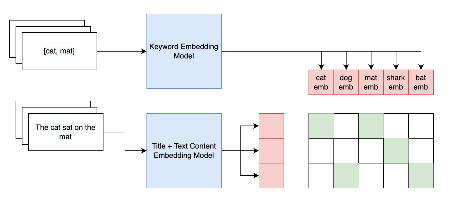
Let's consider an example from the figure above. Suppose we have 3 templates. We pass the text of the template through one sentence transformer and the keywords through another.
Note that even though we have 3 templates we have 5 potential keywords
(cat, dog, mat, shark, bat). Each set of keywords (labels) are
extracted in each batch and are not all possible keywords in that
language.
The green cells represent where there would be a label of 1 and 0 elsewhere. The red cells represent the text representative embeddings. The blue boxes are multilingual sentence transformers(opens in a new tab or window).
The red cells are multiplied together to create a similarity matrix.
Each entry in the matrix is a value between 0 and 1, inclusive of both
values. For instance, in this case if the text embeddings were 3 x 768
and the keyword embeddings were 5 x 768, the similarity matrix would
be 3 x 5. In this example 3 is the batch size while 5 is the
number of keywords found in that batch.
We treat the similarity matrix as logits(opens in a new tab or window), and use a contrastive loss function to train our model. The main distinction with CLIP loss is that the positive labels are only on the diagonal. This does not hold true in our training method.
Data Cleaning, Batching and Mixing Batches
We only use textual features in this model, so this is not a multi-modal model.
The training data that we used was the historical data on templates, the input being the text content of a template while the outputs being the actual keywords. We restrict the training data to our internal creators to ensure a high standard of the model. Unfortunately, external creators have motivation to add irrelevant keywords in order to be visible even in unrelated search queries. While the number of internal creators is far less than the external creators this is of little to no consequence.
In order to get effective training we needed to be careful with how the data was chosen, mixed and batched during training.
To ensure that there were minimal spelling errors in keywords, we chose keywords that appeared at least 30 times across different creators. During training we limit ourselves to the top 1000 keywords per language. This is so that each keyword is seen 'enough' times during the training process. As we shall see soon this 1000 keyword limit does not apply during inference.
Each batch contained one language only. This was done so that at each batch, the keywords come from a single language. This ensures that we do not accidentally give the translated keyword a negative label.
We also observed that the training was worse off if we trained one language and move on to the next. Therefore, we mix the batches randomly so that the model does not get "good" at one language before attempting to move on to the next.
Asymmetric Loss for Ignoring Negative Labels
In the CLIP model, the contrastive loss is specified by the following
pseudocode (taken from Figure 3 in the paper
"Learning Transferable Visual Models From Natural
Language Supervision"(opens in a new tab or window) by Radford et al.), where loss_i and
loss_t represents the loss from learning an image and text
representation respectively.
# symmetric loss functionlabels = np.arange(n)loss_i = cross_entropy_loss(logits, labels, axis=0)loss_t = cross_entropy_loss(logits, labels, axis=1)loss = (loss_i + loss_t)/2
While we can use binary cross entropy loss as above, we found that doing so lead to very poor results. This is likely due to that loss function focusing on trying to push vectors apart for negative labels. This could be simply because there were far more negative labels than positive samples. Triplet loss is a common way to get past this class imbalance. However, this would have involved mining for hard negatives and hard positives for a better classification, which equates to more effort in data collection.
We instead use the Asymmetric
Loss(opens in a new tab or window) which is heavily inspired by focal loss in order to side-step
mining for these hard examples. The bulk of the loss can be explained by
the following equation. The parameter gamma is known as a focusing
parameter, which penalizes hard-to-classify examples relative to
easier-to-classify examples. The asymmetric loss is essentially focal
loss but with a stronger gamma in the negative case. They do also clip
and shift the negative probabilities in order to weaken the effect of
negative examples even more. All of this is so that the model can
automatically focus on the positive examples.
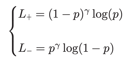
A PyTorch implementation of the loss function code can be seen below.
import torchimport torch.nn as nnimport torch.nn.functional as Fclass AsymmetricLoss(nn.Module):def __init__(self,gamma_neg: float = 4.0,gamma_pos: float = 1.0,clip: float = 0.05,):"""Asymmetric Loss for Multi-label Classification. https://arxiv.org/abs/2009.14119Loss function where negative classes are weighted less than the positive classes.Note: the inputs are logits and targets, not sigmoids.Usage:inputs = torch.randn(5, 3)targets = torch.randint(0, 1, (5, 3)) # must be binaryloss_fn = AsymmetricLoss()loss = loss_fn(inputs, targets)Args:gamma_neg: loss attenuation factor for negative classesgamma_pos: loss attenuation factor for positive classesclip: shifts the negative class probability and zeros loss if probability > clipreduction: how to reduced final loss. Must be one of mean[default], sum, none"""super().__init__()if clip < 0.0 or clip > 1.0:raise ValueError("Clipping value must be non-negative and less than one")if gamma_neg < gamma_pos:raise ValueError("Need to ensure that loss for hard positive is penalised less than hard negative")self.gamma_neg = gamma_negself.gamma_pos = gamma_posself.clip = clipdef _get_binary_cross_entropy_loss_and_pt_with_logits(self, inputs: torch.FloatTensor, targets: torch.LongTensor) -> tuple[torch.FloatTensor, torch.FloatTensor]:ce_loss = F.binary_cross_entropy_with_logits(inputs, targets.float(), reduction="none")pt = torch.exp(-ce_loss) # probability at y_i=1return ce_loss, ptdef forward(self, inputs: torch.FloatTensor, targets: torch.LongTensor) -> torch.FloatTensor:ce_loss, pt = self._get_binary_cross_entropy_loss_and_pt_with_logits(inputs, targets)# shift and clamp (therefore zero gradient) high confidence negative casespt_neg = (pt + self.clip).clamp(max=1.0)ce_loss_neg = -torch.log(pt_neg)loss_neg = (1 - pt_neg) ** self.gamma_neg * ce_loss_negloss_pos = (1 - pt) ** self.gamma_pos * ce_lossloss = targets * loss_pos + (1 - targets) * loss_negreturn loss.mean()
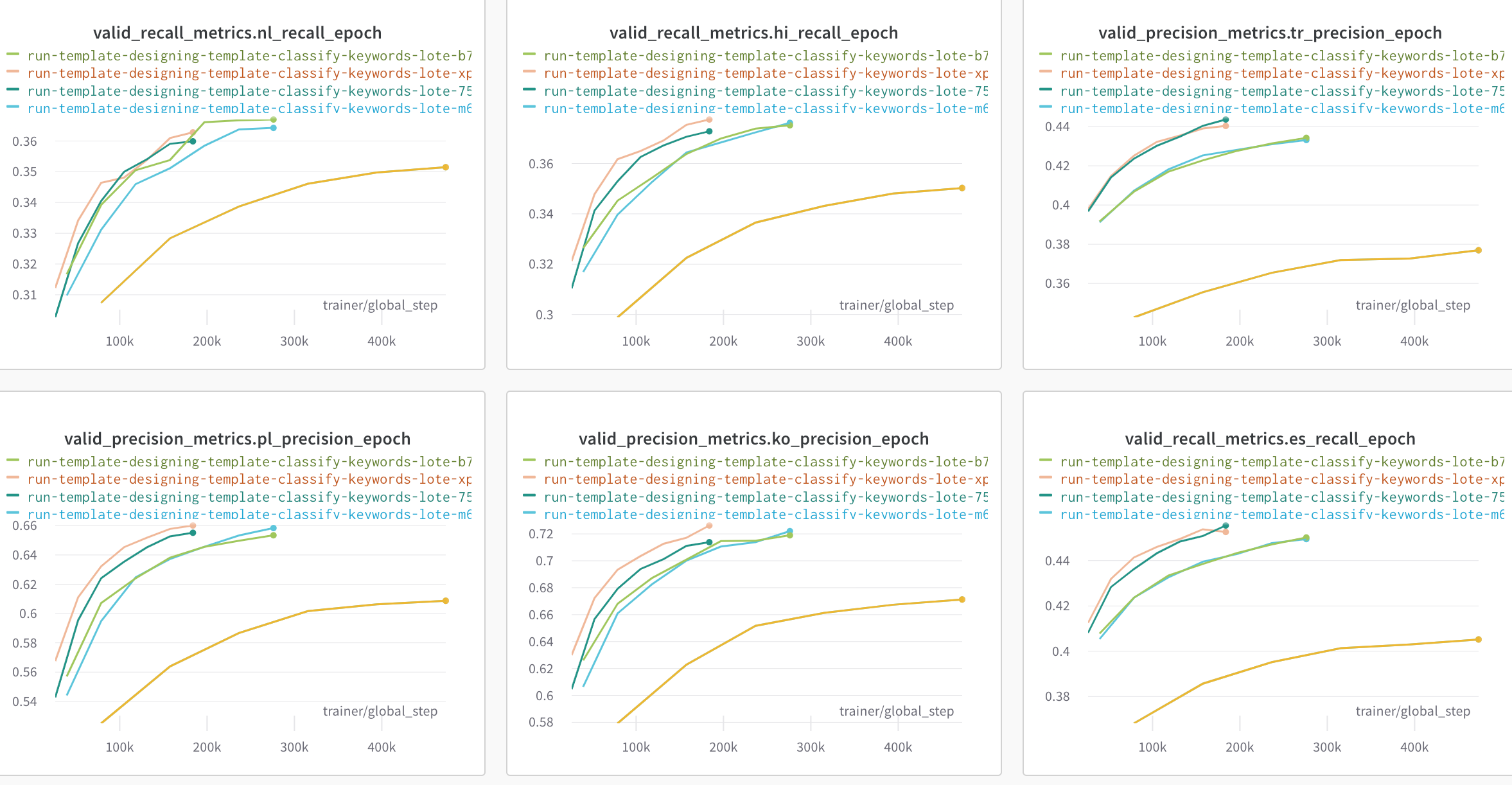
It is worth noting that given that the models (are two pre-trained sentence transformers) even without any training starts off at a good accuracy. The following diagram shows the precision and recall curves for different languages at various hyper-parameters.
Inference
During inference, we take the 1000 most popular keywords per language and serve the 10 highest probability keywords. We further threshold these keywords to ensure only the highest quality keywords are suggested. Given that we are using the asymmetric loss we cannot simply use 0.5, and instead choose a lower value instead. This is due to the fact that, similar to focal loss, the emphasis is on pushing the probability of mislabelled classes higher.
One trick that we use is to precompute the keyword embeddings for all languages for all 1000 keywords. Since the only thing that is dynamic are the template text inputs, we can keep the keyword side constant.
As mentioned earlier, there is nothing stopping us from using unseen keywords during training, or even unseen languages altogether. This is subject to future work.
Summary
In closing, we created a multi-language, multi class classification model. The key ingredients were the twin model, the loss function, and the order in which data was fed into the model.
We are currently serving this model to the thousands of creators that we have. Let us know what you think of our ML models by signing up to Canva Creators(opens in a new tab or window).
Acknowledgements
Huge thanks to Canh Dinh(opens in a new tab or window) for helping to develop and build the model, and Paul Tune(opens in a new tab or window) for helping me in writing this post.
Interested in working on innovative machine learning solutions in design? Join Us!(opens in a new tab or window)


